Posted on November 10, 2021 by Lisa Ward
By Jim Gouveia, Marc Bond, Jeff Brown, Mark Golborne, Bob Otis, Henry S. Pettingill, and Doug Weaver
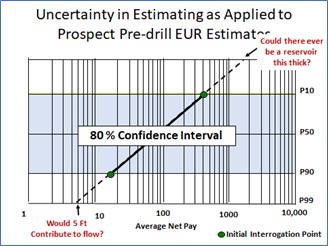
Consider the figure to the right under the lens of predicted net feet of pay. How have you been trained to handle plots such as this one? Here at R&A, we recommend a seven-step approach:
01. Plot the P10 and P90 predictions.
02. Draw a line between the predictions and extrapolate it to the resulting P1 and P99 values.
03. ‘Reality check’ these end members.
On the low end, would the predicted thickness contribute to meaningful sustainable flow? Assuming our area is unknown and highly correlated to our concept of sustainable flow, we get pragmatic and think about the ability to effectively complete the zone, without extraordinary measures. For example, would we be able to effectively complete a 1-foot interval in a homogenous sand which is underlain by 100 ft of water? There is no silver bullet for P99; it will be driven by user experience and play-specific knowledge, with consideration for variables such as permeability, Kv/Kh ratio, depth, infrastructure, viscosity, etc.
One of our biggest challenges when we consider net pay is defining how we differentiate geological successes from commercial successes. (We are talking about the average Net Pay across the productive trap area and not at the planned well location).
On the high end, could one make an optimistic yet realistic prospect map that could house such a thick Average Net Pay? In our collective experience at R&A, the projected P1 value can be unrealistically high—it’s not about the maximum thickness somewhere within the trap, it’s the maximum average thickness across the productive trap area.
04. Adjust the ‘reality check’ high and low members and pragmatically assume these are your new P1 and P99 end members.
05. Plot the ‘reality checked’ P1 and P99 values and redraw the line. The original P10 and P90 values are frequently not preserved and should be thought about as simply serving the purpose of initiating the process. Determine your resulting ‘reality checked’ P10, P50, and P90 values.
06. Inspect your measures of central tendency, the P50, and Mean values. For the P50, ask yourself, “When we think of this prospect, does it feel reasonable that half the time we expect to get a result larger than this value, and half the time less?” In a lognormal distribution, which best characterizes net pay, the P50 is halfway through the frequency, not halfway through the distribution’s parameter values. The Median, which is not synonymous with the P50, is based on sampled data. The reader is advised to always use the P50 which is based on the fitted data. When we are dealing with limited data sets, there can be a significant difference between the Median and the P50.
07. Compare the derived prospect Mean to the distribution of geologically analogous discovered prospects. Predicting a Mean outcome, which lies above the upper ten percent of your analogous discoveries, demands a technically unbiased explanation of why the prospect will have an Average Net Pay that exceeds 90% of the values previously encountered in the play.
Ultimately, exploration organizations need to deliver what they predict, and numerous industry look-back studies have demonstrated that the approach outlined in this example is highly effective in achieving that goal.
The values within our ‘reality checked’ P10 and P90 outcomes represent an “80% confidence interval.” In the E&P industry, we advocate setting the goal for our predictions based upon that range, particularly for the performance of our portfolios (more on that in a later R&A blog).
In a future blog, we will address measures of uncertainty and discuss reality checks based on our ratio of the P10 to P90.
Posted on September 23, 2021 by Lisa Ward
By Jim Gouveia, Marc Bond, Jeff Brown, Mark Golborne, Bob Otis, Henry S. Pettingill, and Doug Weaver
Few industries are fraught with more uncertainty than prospect exploration in E&P. Our formal education guided us with the notion that unless we provide a precise answer, we have ‘failed’ to meet expectations. This is exasperated by investor and leadership’s need for certainty in their investment decisions. When we face an uncertain prediction, we need methods that decouple our minds from trying to jump to ‘the answer’ and instead capture a pragmatic range of possible outcomes.
The present value of our drilling prospects is primarily driven by their probability of realizing commercial success, our corporate discount rate, commodity prices, capital expenses, operating expenses, and our share of the commodity’s cash flow after taxes and royalties. Each of these key parameters is riddled with uncertainty throughout a project’s lifetime.
Modeled ranges better inform decision-makers by fairly representing the spectrum of possible outcomes. Many experts argue that decision-makers simply require confidence in the mean outcome. Portfolio theory advises that given a great number of repeated trials and an unbiased estimation, our firms will deliver the aggregated mean outcome. Whilst portfolio theory is sound, it presupposes two realities that do not exist in the world of exploration. First, our predictions are free of bias. Without a probabilistic basis, grounded by ‘reality checks,’ our forecasts have repeatably proven to be optimistically biased. Second, that there are enough repeated trials to make the aggregate prediction valid over time. No one (especially currently) is drilling enough exploration wells to support high statistical confidence in a program’s ability to deliver a mean outcome.
As decision-makers, we need standardized evaluation techniques upon which we can confidently make our best business investment decisions. That requires that subjective words and phrases such as ‘good chance,’ ‘most likely,’ ‘excellent,’ ‘low risk’ and ‘high confidence’ be eradicated from our presentation of E&P opportunities and replaced with probabilities that have a common definition across all disciplines and projects. The traditional industry consensus is the use of P10 and P90, which in the predominantly used ‘greater than’ convention, represents our optimistic but reasonable high side and our pessimistic but reasonable low side values respectively.
In a prior blog, we introduced our industry-standard method of providing ’P90’ and ‘P10’ values to bracket the ranges of all possible prediction outcomes. Studies have consistently shown that we are not particularly good at making such predictions and tend to underestimate the uncertainty in what we are assessing. For most E&P parameters, this presents itself as having our P10 to P90 ranges too narrow and optimistically high. Until the Petroleum Resources Management System (PRMS) update in 2010, industry guidance for validation of a probabilistic distribution was for the user to compare their probabilistically derived P50 to their deterministic (based upon their best guess) P50. It should not come as a surprise to learn that early probabilistic methods were flawed, as they were based on the belief that in the face of all the inherent subsurface uncertainty, we as subsurface professionals (even those of us who were newly graduated) had an innate ability to directly estimate a P50. Unfortunately, this antiquated belief persists to this day.
So how do we better derive our probabilistic ranges? Let us first bear in mind that we are trying to pragmatically capture the full range of possible outcomes in our predictions. We know that many of our subsurface distributions are often best represented by normal or lognormal distributions. We also know that both normal and lognormal distributions go to positive infinity and that an infinite reserve or rate is neither possible nor pragmatic. On the low end, lognormal distributions approach zero and normal distributions go to negative infinity. At the high end, both lognormal and normal distribution go to infinity. As we are building a distribution to characterize a geological success, we can eliminate the known low and high ends of both distributions either by truncation of outcomes above and below certain thresholds, or our preference at R&A, spike bounding. In spike-bounded distributions, randomly sampled values in excess of the selected high-end limit or low-end limit are respectively set as equal to the selected high- and low-end boundary values. As such the values are ‘bounded’ at the low and high ends of the distribution.
In the exploration realm, we are dealing with a relative dearth of data. Industry experience shows that in the “Exploration space,” we can use the P1 and P99 values of our distributions as the pragmatic end members for our distribution. In practice, we estimate our P90 and P10 values. We then extrapolate these values to a P99 and P1 value. We try to ensure that the P99 value represents the smallest meaningful result – the minimum geological success value – and the P1 value represents the largest geologically defensible result. Our P1 and P99 values are intended to represent a blending of geologic pragmatism and conceptualization. It is a trivial academic debate as to whether these high-end members are or should be our P2, P3 or P0.05 outcomes, the same logic applies to the low-end P99. The use of P1 and P99 should be thought of as a pragmatic spike bounding of the end members (‘reality checks’) of our input distributions.
In summary, our input ranges must capture the entire range of possible outcomes, and industry experience has taught us that to effectivity capture that range, we should consistently employ specifically defined low-side and high-side inputs (e.g., P99, P90, P1, and P10)
In our next article in this series, we will work through an example which addresses Average Net Pay.
Posted on February 17, 2021 by Lisa Ward
by Henry S. Pettingill, Marc Bond, Jeff Brown, Peter Carragher, Mark Golborne, Jim Gouveia, and Bob Otis
One of the common questions that teams ask us when reviewing subsurface projects is, “How should we set our input ranges for volumetrics?” This article introduces a new series that will address that question.
Many published works over the years have documented the importance of predicting what we find for our oil and gas portfolios, in both the exploration and development phases of the project life cycle. While it is impossible to repeatedly find exactly ‘the number’ for every prospect, well, or development, it is possible to get close the prediction on a portfolio basis. The fundamental concept is that for both prospects and portfolios, we can state our prediction in ranges, and additionally in terms of measures of central tendency (our ‘expectation’, commonly the arithmetic mean) and dispersion around that central tendency. The consequence of this latter statement is that we are able to give leadership ‘one number’ for an expectation – which is usually what both the executive suite and the investment community want from us.
So why do we use ranges? Simply put, it has been repeatedly shown that our predictions are better in the long run if, instead of using single values for each input parameter, we employ ranges to ultimately derive confidence intervals and a single value of our ‘expectation’ for that parameter (e.g. Pettingill, 2005). It also makes the elimination of systematic estimating bias more effective, as statistically rigorous post-mortem analyses become possible.
As far as we can tell, the pharmaceutical industry led the way in the 1920s by employing ranges in probabilistic predictions. The first employment of these methods in oil and gas volume prediction was documented in the late 1960s (for instance, Newendorp, 1968).
While most of the major upstream petroleum companies were employing these methods, they advanced and gained wider usage following seminal publications in the 1970s and 1980s by Ed Capen, Pete Rose, Bob Megill, Paul Newendorp, and others (see references below). These references have withstood the test of time and remain relevant today, so we highly recommend reading them.
Later works validated the concepts by demonstrating that pre-drill predictions as a whole were improved with the implementation of probabilistic ranges. These are well documented by Otis and Schneidermann (1997), Johns (1998), Ofstad et al. (2000), McMaster and Carragher (2003) and Pettingill (2005).
Fast forwarding to 2021, what have we observed over the years with respect to the application of these concepts? First, there are still many questions that arise on the topic from the upstream community. Second, some of the digital-era staff have not received an in-depth education on the fundamental concepts that drive input ranges. And finally, it seems like many of us who learned these methods have forgotten some of the fundamentals (or at least become rusty!).
Three fundamental concepts define the modern concepts for pre-drill volumetric assessment: 1) the jump from single deterministic input parameters to probabilistic inputs, 2) the use of continuous probability distributions (e.g., normal, lognormal), and 3) employing confidence intervals associated with these input distributions, and as a consequence, the final output distribution of recoverable resources.
These probabilistic ranges can be characterized by parameters such as probability percentiles (P10, P90, etc.), mean, variance or standard deviation, and P10:P90 ratios (Figure 1). We will expound on these in a future blog. [note: in this blog, we define P10 as high and P90 as low]. The biggest benefit from using these probabilistic ranges is the ability to state our predictions in terms of confidence, e.g. “I have a 90% chance of finding __ mmboe or greater, a 50% chance of getting __ mmboe or greater, and a 10% chance of getting __ mmboe or greater”. Another great advantage is the ability to characterize the distribution with a single mean value or the expectation that encompasses the entire output distribution: the mean, which is the average outcome. This allows us not only to understand the anticipated value of our portfolio as if we drilled our prospect thousands of times but also allows us to objectively compare and rank projects within a portfolio.
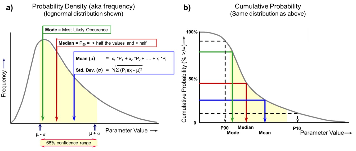
Figure 1. Probability graphs (lognormal distribution shown): a) probability density graph, b) cumulative probability graph. Note that we are using the “greater than or equal to” convention, with P90 as the low-end percentile. The concept applies to both the input parameter as well as the output distribution.
This series will evolve as we go along, so a precise schedule of topics is not set (of course, that will be driven largely by the comments from our readers!). Future topics being contemplated are:
— What should our modeled ranges represent?
— Different approaches to assessing uncertainty in Net Rock Volume (NRV)
— How to handle input parameters that use Averages (net pay, Phi, Sw, etc.)
— How to select ranges in the prospect area
— Spatial Concepts: how to jump from a map to a volumetric input distribution
— Direct Hydrocarbon Indicators (DHIs): specific considerations when choosing volumetric inputs
— Important statistical concepts: Mean, Variance, Standard Deviation, and P10/P90 ratios
We wish to thank all the authors of the works cited here, as well as the countless others not cited, for their contributions to this topic and our industry. They are the true heroes of this journey of learning. We also extend our gratitude to our colleagues at Rose and Associates.
— Capen, E. C. (1976), The difficulty of assessing uncertainty, Journal of Petroleum Technology, August 1976, pp. 843-850.
— Carragher, P. D. (1995), Exploration Decisions and the Learning Organization, Society of Exploration Geophysicists, August 1995, Rio de Janeiro.
— Johns, D. R., Squire, S. G., and Ryan, M. G. (1998), Measuring exploration performance and improving exploration predictions—with examples from Santos’ exploration program 1993-96, APPEA Journal, 1998, pp. 559-569.
— Megill, R. E. (1984), An Introduction to Risk Analysis, 2nd Edition. PennWell Publishing Co. Tulsa.
— Megill, R. E. (1992), Estimating prospect sizes, Chapter 6 in: R. Steinmetz, ed., The Business of Petroleum Exploration: AAPG Treatise of Petroleum Geology, Handbook of Petroleum Geology, pp. 63-69.
— McMaster, G. E. and Carragher, P. D. (1996), Risk Assessment and Portfolio Analysis: the Key to Exploration Success. 13th Petroleum Conference, Cairo Egypt, 1996.
— McMaster, G. E. and Carragher, P. D. (2003), Fourteen Years of Risk Assessment at Amoco and BP: A Retrospective Look at the Processes and Impact, Canadian Society of Petroleum Geologists / Canadian Society of Exploration Geophysicists 2003 Convention, Calgary Alberta, June 2-6.
— Newendorp, P. (1968). Risk analysis in drilling investment decisions. J. Petroleum Technology, Jun. pp. 579-85.
— Ofstad, K., Kittilsen, J.E., and Alexander-Marrack, P., eds. (2000), Improving the Exploration Process by Learning from the Past, Norwegian Petroleum Society (NPS) Special Publication no. 9. Elsevier, Amsterdam, 279 p.
— Otis, R. M., and Schneidermann, N. (1997), A Process for Evaluating Exploration Prospects, AAPG Bulletin v. 81, No. 7, pp 1087-1109.
— Pettingill, H.S. (2005) Delivering on Exploration through Integrated Portfolio Management: the Whole is not just the Sum of the Holes. SPE AAPG Forum, Delivering E&P Performance in the Face of Risk and Uncertainty: Best Practices and Barriers to Progress. Galveston, Texas, Feb. 20-24, 2005.
— Rose, P. R., (1987), Dealing with risk and uncertainty in exploration: how can we improve?, AAPG Bulletin, vol. 71, no. 1, pp. 1-16.
— Rose, P. R. (2000), Risk Analysis in Petroleum Exploration. American Association of Petroleum Geologists.